

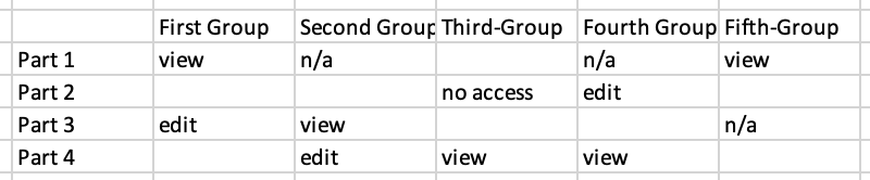
So here's a thing I needed to do in Excel. I received a table in a task at work, with a matrix of different user groups and their access rights to different parts of our app. If I simplify it and remove all sensitive data, it looked like this:
To simplify coding I wanted a column where all relevant roles would be listed, ready for copy-pasting into the code. So here's how I went about doing this.
Firstly
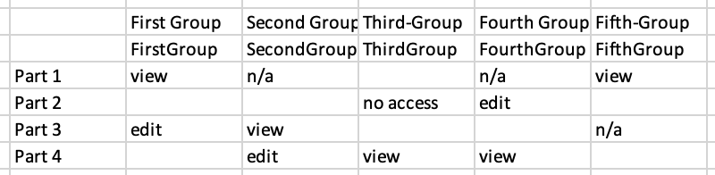
I created a separate row under the group names, to remove unnecessary spaces and dashes with the following formula: =SUBSTITUTE(SUBSTITUTE(H6;" ";"");"-";""), receiving this:
And the most exciting part was learning to use array formulas and TEXTJOIN to create conditioned concatenations, building strings with groups that I needed. The key to understanding this is the following: IF can receive ranges in its arguments when used in an array formula. To create an array formula, instead of confirming the formula entry with Return, press Ctrl+Shift+Return (on a Mac), which results in the formula getting enclosed in curly brackets.
The bad thing is you cannot use AND() in array functions, so instead of AND() you have to use nested IF()s. So, to filter out blanks, n/a's and no accesses we need the following: =IF(NOT(H8:L8="n/a");IF(NOT(H8:L8="no access");IF(NOT(H8:L8="");$H$7:$L$7;"");"");""). It checks the range for n/a, and if it is not found, checks for no access, if that is not found either, it checks for a blank. If none of those three is found, it references the corresponding cell in the row with group names with removed spaces through $H$7:$L$7, where $ means that I always want to reference that range, even when copy-pasting the formula.
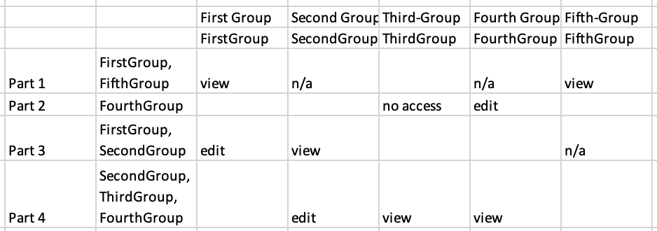
This won't work yet though. To finish off the formula, we have to use TEXTJOIN(). It accepts 3+ arguments, where the first one is a delimiter, second is a boolean that determines whether blanks have to be concatenated or not, and the other arguments are arrays that have to get concatenated. So, we have to enclose our large IF() into TEXTJOIN(", ", TRUE, IF), creating this beauty: =TEXTJOIN(", ", TRUE, IF(NOT(H8:L8="n/a");IF(NOT(H8:L8="no access");IF(NOT(H8:L8="");$H$7:$L$7;"");"");"")). Don't forget to confirm with a Ctrl+Shift+Return press:
Secondly
Then I realized that I don't really need the row where I substituted out all those spaces and dashes, and I incorporated the SUBSTITUTE() into TEXTJOIN(), resulting in this: =TEXTJOIN(", ", TRUE, IF(NOT(H8:L8="n/a");IF(NOT(H8:L8="no access");IF(NOT(H8:L8="");SUBSTITUTE(SUBSTITUTE($H$7:$L$7;" ";"")"-";"");"");"");"")) Another press of Ctrl+Shift+Return, and we're golden.